A little background

Back in college, I played a lot of puzzle games. When I talk about these kinds of games, I'm going to be referring to a very specific subset of puzzle game. Some examples include:

• Stephen's Sausage Roll
• English Country Tune
• Sokobond

I was also fortunate to take Data Structures at RPI, where at the time professor Cutler (hi Barb!) had a yearly assignment/competition where students to write a puzzle solver. The game changed every year, and for my year the game was Ricochet Robots, which is essentially a sliding ice puzzle with multiple players. I really enjoyed the assignment (and won the competition!) and continued to enter the competition as a TA. I probably went too hard on it in retrospect; hopefully I wasn't too much of a nuisance!

Anyway, the purpose of the assignment was to get everyone familiar with recursion and depth-first search. Your program would be given the initial state of the game as well as a maximum recursion depth. The goal was to return either the shortest possible solution, or all possible solutions of minimum length. For the competition, you may or may not be passed a depth limit and might also be given puzzles that had no solution. I learned a lot and had a lot of fun, so maybe you will too.

Abstract

In this article, I will present a new puzzle game and demonstrate techniques I used to write a fast, practical solver for it. Topics covered will include breadth-first/A* search, memoization, optimization, and strategies specific to NP-hard and NP-complete puzzle games. If you spot any problems or want to suggest any improvements, please file an issue or submit a PR on GitHub. I will present benchmarks to validate my results throughout. While the percentage changes should be relatively accurate, the absolute timings may vary throughout as they are taken at different times with different amounts of baseline noise. The pre-/post- change benchmarks are always run back-to-back to ensure that they are run in the same environment and provide accurate percentage change.

Let's play a game

The game we're going to play is called "Anima". It uses a grid of tiles, each of which is either passable or impassable. Some tiles are marked with a small colored diamond; these tiles are goals and to solve the puzzle we have to cover all of these tiles simultaneously with actors of the same color. Actors are blocks, at most one per tile, that can be moved around the grid on the passable tiles. Each turn, you may move the actors in one of the four cardinal directions and they all slide together. Let's do a few to get a feel for it:

These two are pretty easy, but you might have noticed some implicit rules that make solving these puzzles nontrivial:

• If an actor tries to move into an impassable tile, they do not move.
• If an actor would overlap another actor, they do not move.

These side-effects make it very difficult (impossible?) to predict how the system will behave after even a move or two, which is a hallmark of problems with high NP-complexity. We'll add one more twist to make it a little more interesting:

Unlike red actors, blue actors move in the opposite direction you choose. If you choose left, blue actors will move right and vice-versa. This leads to one final implicit rule:

When they're right next to each other, red and blue actors can pass through each other to exchange positions. However, if they're separated by a single space, they'll try to move onto the same space and block each other from moving at all. This added complexity can make puzzles much more difficult to solve.

Before diving in, I'd definitely recommend trying out some more puzzles to get a better feel for some high-level techniques and to get better acquainted with the game. Don't worry about solving all of these, they can get very hard. Just work with them until you feel competent and confident.

This is where we start writing our solver. You can follow along using the start tag on the GitHub repo, which will start you with all of the boilerplate:

git clone --branch start https://github.com/djkoloski/anima_solver

A basic solver

Our strategy for a basic solver will be to explore, one move at a time, out from the initial state until we find a solution. I'll do this with a basic breadth-first search augmented with parent tracking:

pub fn solve(initial_state: State, data: &Data) -> Option<Vec<Direction>> {
    let mut parents = Vec::new();
    let mut queue = VecDeque::new();

    // Add transitions from initial state
    for (action, transition) in initial_state.transitions(data) {
        match transition {
            Transition::Indeterminate(state) => {
                parents.push((0, action));
                queue.push_back(state);
            }
            Transition::Success => return Some(vec![action]),
        }
    }

    // Pop states in order
    let mut index = 0;
    while let Some(parent_node) = queue.pop_front() {
        index += 1;

        for (action, transition) in parent_node.transitions(data) {
            match transition {
                Transition::Indeterminate(state) => {
                    parents.push((index, action));
                    queue.push_back(state);
                }
                Transition::Success => {
                    let mut result_actions = vec![action];
                    let mut current_index = index;
                    while current_index != 0 {
                        let (next_index, action) = parents.swap_remove(current_index - 1);
                        result_actions.push(action);
                        current_index = next_index;
                    }
                    result_actions.reverse();
                    return Some(result_actions);
                }
            }
        }
    }

    None
}

There's a lot of boilerplate omitted, so here's what's relevant:

• We have State and Data structs where State is all the information that can change and Data is all the information that is static. State is the positions of the actors, and Data is the layout of the board and goal positions. These are separated out to minimize how much memory is being used by queue.
• The transitions() method operates on a State, takes some Data, and returns the new states we reach by performing every possible move. An Indeterminate transition means that the state you reach is not solved, and a Success transition means that it is.

parents here is a list of (usize, Direction) that tracks what state it came from and what direction was moved to transition. When we get a successful transition, we crawl back through the parents vector to reassemble the solution and return it. Let's try it out!

We're going to use a nice and simple one to test:

$ cargo run -- puzzles/line_dance.txt
puzzles/line_dance.txt:
Parse: 0.000201900s
Solve: 0.000017600s
Found solution of length 2:
Right, Right

Cool, it found it! And that looks right too, let's see how fast it is in release mode:

$ cargo run --release -- puzzles/line_dance.txt
puzzles/line_dance.txt:
Parse: 0.000122700s
Solve: 0.000009100s
Found solution of length 2:
Right, Right

Roughly twice as fast, great! We're going to be running exclusively in release mode from here on out. Now let's step it up a little bit and try a harder puzzle:

$ cargo run --release -- puzzles/u_turn.txt
puzzles/u_turn.txt:
Parse: 0.005942000s
Solve: 0.001093200s
Found solution of length 6:
Down, Down, Left, Left, Up, Up

Awesome, it got that one too! One more, this one's really more of the same:

$ cargo run --release -- puzzles/spiral.txt
...

Uh oh, this one doesn't seem to be going anywhere fast. And if you don't kill it soon, you might run out of memory too! Looking at the timings explains why:

puzzles/line_dance.txt
Solve: 0.000009100s
Found solution of length 2:

puzzles/u_turn.txt
Solve: 0.001093200s
Found solution of length 6:

By adding just four moves to the solution length, our runtime went up by a factor of 120x! Let's take a peek at how many states we're exploring:

println!("Explored {} states", parents.len());

$ cargo run --release -- puzzles/line_dance.txt
Explored 3 states

$ cargo run --release -- puzzles/u_turn.txt
Explored 5364 states

Yikes, there's our problem. And it makes sense, every state we explore leads to four more states so we should expect that a solution of length n will explore at least (4^n - 1) / 3 states. For a 6-move solution, that comes out to between 1365 and 5461 states, so we're right in that range. What does that mean for our currently-unsolvable puzzle? It takes 16 moves to solve it, so we should expect to explore between 1431655765 and 5726623061 states.

Uh oh.

Now it's time to start iterating on our solver and improving it. We will measure progress by measuring how long it takes to solve existing puzzles, then creating new and more difficult puzzles as we go along. Our goal will be to quickly solve all puzzles that we can create.

State tracking

First, we should observe that even though we explored 5364 states for U-Turn, there are functionally only seven unique states: one for each of the tiles the actor could be on. So we must be exploring the same state multiple times. We can avoid this by storing our explored states in a hash set and only exploring its children if it's not already been visited:

let mut states = HashSet::new();
...

while let Some(parent_node) = queue.pop_front() {
    index += 1;

    if !states.contains(&parent_node) {
        ...

        states.insert(parent_node);
    }
}

Let's see how this affects our cases so far:

$ cargo run --release -- puzzles/u_turn.txt
Explored 20 states
Solve: 0.000895100s
Found solution of length 6:   
Down, Down, Left, Left, Up, Up

That looks much better! Maybe we can solve our new puzzle now?

$ cargo run --release -- puzzles/spiral.txt
Explored 51 states
puzzles/spiral.txt:
Parse: 0.000212300s
Solve: 0.001049000s
Found solution of length 16:
Left, Left, Up, Up, Right, Right, Right, Right, Down, Down, Down, Down, Left, Left, Left, Left

That's much better, bringing our explored states down from over a billion to just 51. This optimization alone brings all our sample puzzles into the realm of solvability! Now we can start benchmarking our solver more comprehensively. Let's pick a few representatives from the sample puzzles set to bench:

$ cargo bench
solve_square_dance      time:   [16.658 ms 16.888 ms 17.125 ms]
solve_fractal           time:   [44.606 ms 45.193 ms 45.806 ms]
solve_antiparticle      time:   [1.8001 s 1.8308 s 1.8640 s]

Entropy reduction

One easy optimization we can make is to reduce the entropy of our states. Right now our puzzle state looks like this:

enum Color {
    Red,
    Blue,
}

pub struct Actor {
    position: Vec2,
    color: Color,
}

pub struct State {
    actors: Vec<Actor>,
}

So imagine a board with a few red actors on it. Let's say four, labeled A, B, C, and D:

With these four actors, there's actually 4! ways we could represent the state since there are 4! permutations of the actors in the vector. We can fix this by sorting our actors array. This will reorder any permutation of the actors into one canonical ordering. We can do this pretty easily when we transition our states:

pub fn transition(&self, data: &Data, direction: &Direction) -> State {
    let mut result = self.clone();

    ...

    result.actors.sort();
    result
}

A good way to think of this is as removing any unnecessary entropy in the state. Let's see how that affects our benchmarks:

$ cargo bench

solve_square_dance      time:   [4.4875 ms 4.5667 ms 4.6525 ms]
                        change: [-73.527% -72.960% -72.308%] (p = 0.00 < 0.05)

solve_fractal           time:   [19.518 ms 19.647 ms 19.776 ms]
                        change: [-57.178% -56.527% -55.885%] (p = 0.00 < 0.05)

solve_antiparticle      time:   [187.49 ms 190.53 ms 193.91 ms]
                        change: [-89.835% -89.593% -89.343%] (p = 0.00 < 0.05)

Let's see how the number of states explored (and branching factor) changed with that:

Puzzle	Solution Length	Before (BF)	After (BF)	Change
Square Dance	12	37268 (2.292)	11401 (2.061)	-61.408%
Fractal	13	86277 (2.294)	46253 (2.179)	-46.390%
Antiparticle	22	2514936 (1.888)	315100 (1.708)	-87.471%

Getting big performance improvements from small changes like this is what we're aiming to do most of the time. The important thing here is that by reducing our state entropy, we reduced our branching factor by a little bit. That small change amplifies quickly in exponential algorithms, so even a very small decrease can lead to huge improvements.

A* search

With that in mind, one easy way we can decrease our branching factor even more is by using a more sophisticated searching algorithm. A* is a very common augmentation to breadth-first search that prioritizes exploring more promising nodes first. In practice, this means that we have to define a heuristic function that estimates the minimum number of moves to completion. We want our heuristic function to estimate the remaining distance as closely as possible, but never overestimate. It's okay to underestimate. With this estimate of the number of moves remaining, we prioritize exploring states that have the minimum estimated solution size (moves so far + remaining moves). This can help us avoid exploring states that are clearly dead ends and prioritize states that look promising.

The main difficulty with implementing A* is determining a good heuristic function. A good heuristic function should be easy to compute and return an estimate that is as high as possible without overestimating. This is a tradeoff that we actively have to be conscious of. In most cases, it will be a net positive. Let's think about what heuristics we can calculate for our puzzle:

In order to complete the puzzle, each goal needs one actor of its color on top of it. Since all the actors move at the same time, we can use a straightforward maxmin: Find the nearest actor to each goal and calculate the distance between them, then take the maximum value of all goal distances. The logical way to think about this is that we're calculating the minimum number of moves necessary to get any actor of our choice to any given goal. This is an extremely rough estimate, but it will work for us. If we wanted, we could calculate the assignment bottleneck instead, but that could take a lot of time and negatively impact our performance. Also UPS lost my book from SIAM.

pub fn heuristic(&self, data: &Data) -> usize {
    let mut max_distance = 0;

    for goal in data.goals.iter() {
        let mut min_distance = usize::MAX;
        for actor in self.actors.iter().filter(|a| a.color == goal.color) {
            let d = (goal.position - actor.position).abs();
            min_distance = usize::min(min_distance, (d.x + d.y) as usize);
        }
        max_distance = usize::max(max_distance, min_distance);
    }

    max_distance
}

Does what it says on the tin. The more difficult part is adapting our existing solve function to prioritize states and calculate the heuristic. The first change we'll make is to bundle all of the information we need when exploring a node into a new structure:

#[derive(Eq, PartialEq)]
struct Node {
    state: State,
    distance: usize,
    estimate: usize,
    index: usize,
}

This will be what we insert into our queue now. Speaking of which:

let mut queue = BinaryHeap::new();

A BinaryHeap is a simple data structure that we can use as a priority queue. We can insert items and remove the maximum value in log(N) time. All we need to do is define an ordering on our nodes that gives the most promising nodes (with lowest distance + heuristic) the highest priority:

impl PartialOrd for Node {
    fn partial_cmp(&self, other: &Self) -> Option<Ordering> {
        Some(self.cmp(other))
    }
}

impl Ord for Node {
    fn cmp(&self, other: &Self) -> Ordering {
        other.estimate.cmp(&self.estimate)
    }
}

A little opaque, but this just says that we want to sort in reverse estimate order. Finally, we need to change our push operation to account for the new fields we need to fill out in Node:

let estimate = state.heuristic(data) + (parent_node.distance + 1);
queue.push(Node {
    state: state,
    distance: parent_node.distance + 1,
    estimate,
    index: parents.len(),
});

Instead of counting our states as we pop them off, we now need to keep track of which index our current state is in the parents list. And with that, we're done! We have a fully-functional A* implementation ready to make our solver go super fast!

$ cargo bench

solve_square_dance      time:   [4.4051 ms 4.4276 ms 4.4524 ms]
                        change: [+3.7025% +4.6095% +5.4779%] (p = 0.00 < 0.05)

solve_fractal           time:   [7.7314 ms 7.7718 ms 7.8183 ms]
                        change: [-57.412% -57.044% -56.682%] (p = 0.00 < 0.05)

solve_antiparticle      time:   [201.26 ms 202.26 ms 203.36 ms]
                        change: [+14.570% +15.351% +16.121%] (p = 0.00 < 0.05)

Well that's a little disappointing. At least, it is if you only look at the individual benchmarks. Two went up by around 5-15%, and one went down by over 50%. So while it wasn't a unilateral gain, it did give us a net benefit overall. And now, if we can improve our heuristic function somehow we can gain the benefit from that too. Let's take a look at our explored states (and branching factor):

Puzzle	Solution Length	Before (BF)	After (BF)	Change
Square Dance	12	11401 (2.061)	9737 (2.031)	-14.595%
Fractal	13	46253 (2.179)	16593 (2.002)	-64.126%
Antiparticle	22	315100 (1.708)	269211 (1.695)	-14.563%

It's important to remember to benchmark very carefully, since even though our states explored fell for every puzzle, our total runtime did increase for two of them. Also a very small change in the branching factor for Fractal resulted in a massive decrease in explored states. The average runtime has fallen quite nicely.

Reducing allocations

The first rule of high-performance optimization is to reduce your allocations. Let's take a look and see if there are some places we can do that:

pub fn transitions(&self, data: &Data) -> Vec<(Direction, Transition<Self>)> {
    ...
}

Our transitions function is returning a Vec with data allocated on the heap, but we know that we'll always return four transitions. We can make this return an array instead:

pub fn transitions(&self, data: &Data) -> [(Direction, Transition<Self>); 4] {
    ...
}

Let's see what that gets us:

$ cargo bench

solve_square_dance      time:   [4.4052 ms 4.4415 ms 4.4867 ms]
                        change: [-7.0971% -6.1140% -4.9385%] (p = 0.00 < 0.05)

solve_fractal           time:   [7.6836 ms 7.7682 ms 7.8720 ms]
                        change: [-8.5312% -7.0938% -5.5943%] (p = 0.00 < 0.05)

solve_antiparticle      time:   [207.00 ms 207.71 ms 208.44 ms]
                        change: [-4.9600% -4.2495% -3.5907%] (p = 0.00 < 0.05)

Some modest gains, let's keep going. Next we can use the arrayvec crate to reduce the number of allocations in our states. It's essentially an inline-allocated array structure, so we won't constantly be allocating heap memory as long as we can put an upper bound on the number of actors in our puzzles. Let's pick eight for some headroom:

pub struct State {
    actors: ArrayVec<Actor, 8>,
}

How about that:

$ cargo bench

solve_square_dance      time:   [4.0299 ms 4.0567 ms 4.0854 ms]
                        change: [-9.7690% -8.6635% -7.6778%] (p = 0.00 < 0.05)

solve_fractal           time:   [7.4610 ms 7.5152 ms 7.5743 ms]
                        change: [-4.6656% -3.2571% -1.9086%] (p = 0.00 < 0.05)

solve_antiparticle      time:   [187.27 ms 188.29 ms 189.38 ms]
                        change: [-9.9536% -9.3494% -8.7499%] (p = 0.00 < 0.05)

Nice! Some more modest gains, but every bit helps. It's finally time to move on to...

Profiling

We're out of low-hanging fruit, so let's move on to doing some micro-optimization. There's still plenty to be gained here though, and we can find it by doing some profiling. Running our benchmarks in Visual Studio gets us some interesting insights:

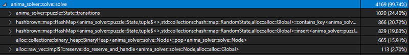
Here they are typed out:

Function	Total CPU %
anima_solver::puzzle::State::transitions	24.40%
hashbrown::map::HashMap::contains_key	20.72%
hashbrown::map::HashMap::insert	19.83%
alloc::collections::binary_heap::BinaryHeap::pop	15.91%

One thing that immediately jumps out is that we're spending almost the same amount of time in HashMap::contains_key as we do in HashMap::insert. But we don't have any hash maps in our solver, do we?

Well actually, we do. We're using a HashSet for our visited states, and that's secretly a HashMap<K, ()> under the hood. Let's take a look at our code:

let mut states = HashSet::new();

...

while let Some(parent_node) = queue.pop() {
    if !states.contains(&parent_node.state) {
        for (action, transition) in parent_node.state.transitions(data) {
            ...
        }
        states.insert(parent_node.state);
    }
}

So there's the problem, we're checking to see if the set contains the state, then getting our transitions, and after that we're inserting the state. We should be able to use an Entry API to check if the set contains the state and insert it with a single lookup right? Well... HashSet doesn't have an entry API like HashMap does yet. Well, I guess we can use a HashMap with a value of () right?

let mut states = HashMap::new();

...

while let Some(parent_node) = queue.pop() {
    if let Entry::Vacant(entry) = states.entry(parent_node.state) {
        for (action, transition) in entry.key().transitions(data) {
            ...
        }
        entry.insert(());
    }
}

That should do the trick. Let's see how that changed our runtime:

$ cargo bench

solve_square_dance      time:   [3.8785 ms 3.9364 ms 3.9998 ms]
                        change: [+0.9796% +2.8698% +4.8065%] (p = 0.00 < 0.05)

solve_fractal           time:   [6.7915 ms 6.8446 ms 6.9022 ms]
                        change: [-2.2994% -1.2597% -0.0914%] (p = 0.03 < 0.05)

solve_antiparticle      time:   [172.04 ms 172.76 ms 173.54 ms]
                        change: [-2.4655% -1.8303% -1.1884%] (p = 0.00 < 0.05)

Well that's disappointing, there's statistically no change in runtime. I guess the entry API must have some overhead that's just as expensive as a lookup and insert. If anyone has ideas on why this didn't change the overall runtime, I'd love to know. But this also shows the importance of benchmarking every step of the way. Even the most obvious improvements can end up having no effect on the overall performance, or worse a negative impact.

Container pre-sizing

We're getting close to the bottom of the barrel. A quick and easy optimization we can do is to pre-size our containers. This helps us skip any work we might do to resize containers for work loads under some minimum size. I've picked some relatively arbitrary pre-sizes here:

let mut states = HashMap::with_capacity(4 * 1024);
let mut parents = Vec::with_capacity(4 * 1024);
let mut queue = BinaryHeap::with_capacity(1024);

We should expect these to only impact any puzzles that don't use memory above the pre-sizing threshold. Do we?

$ cargo bench

solve_square_dance      time:   [3.7025 ms 3.7311 ms 3.7652 ms]
                        change: [-9.7612% -8.3409% -6.9754%] (p = 0.00 < 0.05)

solve_fractal           time:   [6.0512 ms 6.1010 ms 6.1584 ms]
                        change: [-15.633% -14.231% -12.778%] (p = 0.00 < 0.05)

solve_antiparticle      time:   [177.28 ms 178.40 ms 179.59 ms]
                        change: [-0.7913% +0.0458% +0.8882%] (p = 0.92 > 0.05)

That's exactly what we see. We do get some very nice deltas on our smaller puzzles, but our larger puzzle benchmark is completely unaffected. Still, it's bringing down our average case and that's important for us. Finally, we can move on to the last optimization strategy:

Inlining

One of the last tools in our performance toolbox is function inlining. The impact of function inlining varies widely, and we should always be careful to benchmark our code along the way. Let's see if there are any good candidates for inlining. Ideally, a good function to inline should either be small or medium-sized and used once or twice. We have a lot of basic little functions in our vector and direction primitives that we can inline, so those might help a little. Inlining our especially hot transition function for our puzzle state should also help eliminate some overhead. Let's see how that impacts our performance:

$ cargo bench

solve_square_dance      time:   [3.7629 ms 3.8005 ms 3.8413 ms]
                        change: [-10.293% -8.6516% -6.9645%] (p = 0.00 < 0.05)

solve_fractal           time:   [6.7174 ms 6.8059 ms 6.9033 ms]
                        change: [-10.243% -8.5148% -6.7086%] (p = 0.00 < 0.05)

solve_antiparticle      time:   [175.97 ms 176.63 ms 177.38 ms]
                        change: [-6.8481% -5.9110% -5.0767%] (p = 0.00 < 0.05)

A final solid set of improvements! It's always nice to see. Let's wrap up with some final thoughts.

Wrap up

We've successfully made a puzzle solver that's capable of solving all of our given inputs and optimized it using techniques specific to brute-forcing as well as general optimization techniques. We looked at the performance impacts of various techniques and know what to expect in the future. Finally, we also learned not to assume that any particular optimization will affect every case evenly, or even positively.

In the future, the best gains will likely come from improving our heuristic function. For this relatively simple game, there might not be much of a better heuristic we can calculate. In a more complex game, we can often leverage the information in the puzzle to make a much better function though. When writing a solver for Stephen's Sausage Roll, which permitted a more accurate heuristic, the gains from a heuristic function were much larger.

Finally, you can actually use the solver written here right now! You can turn on the solver for any page that has a puzzle on it by adding &controls=true to the URL (here for example). Here's one with the solver enabled, try it out! You can also write, import, and share your own puzzles.

Thanks for reading, and happy solving!